18 - Conduction - Unsteady Heat Conduction

If the lumped capacitance approximation can not be made, consideration must be given to spatial, as well as temporal, variations in temperature during the transient process.

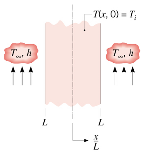
For slab of of thickness \(2L\), considering symmetry with respect to \(x=0\) at the midplane, with constant \(k\), and no heat generation, we have \[\frac{\partial^2T}{\partial x^2} = \frac{1}{\alpha}\frac{\partial T}{\partial t} \qquad \text{ in } 0< x < L, \text{ for } t > 0\]

Slab

Boundary and Initial Conditions: \[\begin{aligned} {3} \frac{\partial T}{\partial x} &=0 \qquad & & \text{ at } x = 0, \text{ for } t > 0 \\ k\frac{\partial T}{\partial x} + h T &= hT_\infty & & \text{ at } x = L, \text{ for } t > 0 \\ T &= T_i & & \text{ for } t = 0, \text{ in } 0 \le x \le L \end{aligned}\]

Dimensionless Quantities: \[\begin{aligned} {3} \theta &= \frac{T(x,t)-T_\infty}{T_i-T_\infty} \qquad & & \text{dimensionless temperature} \\ X &= \frac{x}{L} & & \text{dimensionless coordinate} \\ \text{Bi} &= \frac{hL}{k} & & \text{Biot number} \\ \tau &= \frac{\alpha t}{L^2} & & \text{dimensionless time, or Fourier number} \end{aligned}\]