Instant Notes: 5. Stability Analysis
5.3 Frequency Response Analysis of Linear Processes
-
Basis of frequency response analysis
-
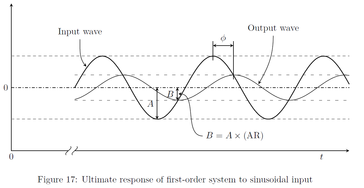
When a linear system is subjected to a sinusoidal input, its ultimate response (i.e., it’s response after a long time) is also a sustained sinusoidal wave. This characteristic constitutes a basis of frequency response analysis.
Refer to Fig.(17).
-
In this analysis, the focus of interest is on how the amplitude ratio (AR) and phase shift (\(\phi\)) of output sinusoidal wave change with the frequency (\(\omega\)) of input sinusoid.
-
The amplitude ratio (AR) and phase shift \(\omega\) of linear systems are obtained by the modulus and argument of the transfer function, with the substitution of \(s = j\omega\).
-
For a complex number \(Z\) defined by \[Z = x + j y\] modulus of \(Z\) represented by \(|Z|\) is obtained by \[|Z| = \sqrt{[\text{Re}(Z)]^2+[\text{Im}(Z)]^2} = \sqrt{x^2+y^2}\] and, the argument of complex number \(Z\) represented by \(\angle Z\) is obtained from \[\angle Z = \tan^{-1}\left[\frac{\text{Im}(Z)}{\text{Re}(Z)}\right] = \tan^{-1}\left(\frac{y}{x}\right)\]
System Transfer function Amplitude ratio (AR) Phase shift (\(\phi\)) First order \(\displaystyle \frac{K_p}{\tau_p s+1}\) \(\displaystyle \frac{K_p}{\sqrt{\tau_p^2\omega^2+1}}\) \(\displaystyle \tan^{-1}(-\omega \tau_p)\) Pure capacitive \(\displaystyle \frac{K_p}{s}\) \(\displaystyle \frac{K_p}{\omega}\) \(-90^o\) Dead time \(\displaystyle e^{-\tau_d s}\) 1 \(-\tau_d \omega\) Second order \(\displaystyle \frac{K_p}{\tau^2s^2+2\zeta\tau s+1}\) \(\displaystyle \frac{K_p}{\sqrt{(1-\tau^2\omega^2)^2+(2\zeta\tau\omega)^2}}\) \(\displaystyle \tan^{-1}\left(-\frac{2\zeta\tau\omega}{1-\tau^2\omega^2}\right)\) Proportional controller \(K_c\) \(K_c\) 0 PI controller \(\displaystyle K_c\left(1+\frac{1}{\tau_I s}\right)\) \(\displaystyle K_c\sqrt{1+\frac{1}{(\omega\tau_I)^2}}\) \(\displaystyle \tan^{-1}\left(\frac{-1}{\omega\tau_I}\right)\) PD controller \(K_c(1+\tau_Ds)\) \(K_c\sqrt{1+\tau_D^2\omega^2}\) \(\tan^{-1}(\tau_D\omega)\) PID controller \(\displaystyle K_c\left(1+\frac{1}{\tau_Is}+\tau_Ds\right)\) \(\displaystyle K_c\sqrt{\left(\tau_D\omega-\frac{1}{\tau_I\omega}\right)^2+1}\) \(\displaystyle \tan^{-1}\left(\tau_D\omega-\frac{1}{\tau_I\omega}\right)\) Systems in series \(G_1(s)G_2(s)\cdots G_N(s)\) (AR)\(_1\)(AR)\(_2\cdots\)(AR)\(_N\) \(\phi_1+\phi_2+\cdots+\phi_N\) First order plus dead time \(\displaystyle \frac{K_pe^{-\tau_ds}}{\tau_ps+1}\) \(\displaystyle \frac{K_p}{\sqrt{\tau_p^2\omega^2+1}}\) \(\displaystyle \tan^{-1}(-\omega \tau_p)-\tau_d\omega\) -
-
The above table gives the values of amplitude ratio and phase shift of various systems for sinusoidal input of \(\sin(\omega t)\). Zeros at the origin, cause a constant \(+90^\circ\) phase shift for each zero. Poles at the origin, cause a constant \(-90^\circ\) phase shift for each pole.