Instant Notes: 5. Stability Analysis
-
Nyquist Plots
-
Nyquist plot is an alternate to Bode plot, and contains the same information as the pair of Bode plots.
-
It has \(\text{Im} [G(j\omega)]\) as ordinate and \(\text{Re} [G(j\omega)]\) as abscissa.
-
A specific value of the frequency \(\omega\) defines a point on this plot. A curve for the variation of \(\omega\) from 0 to \(\infty\) is drawn. The distance of the point in the curve from the origin \((0,0)\) is the amplitude ratio at the frequency \(\omega\). The angle \(\phi\) with the positive real axis is the phase shift at the frequency \(\omega\).
-
The construction of Nyquist plot may be done as follows:
-
For a given transfer function, substitute \(s = j \omega\)
-
Find the AR and \(\phi\) by guessing various values for frequency (\(\omega\)).
-
Calculate \((x,y)\) data as follows:
\[x = \text{AR} \cos(\phi) \qquad y= \text{AR} \sin(\phi)\]
-
Plot this \((x,y)\) data on a graph paper to obtain the Nyquist plot.
-
-
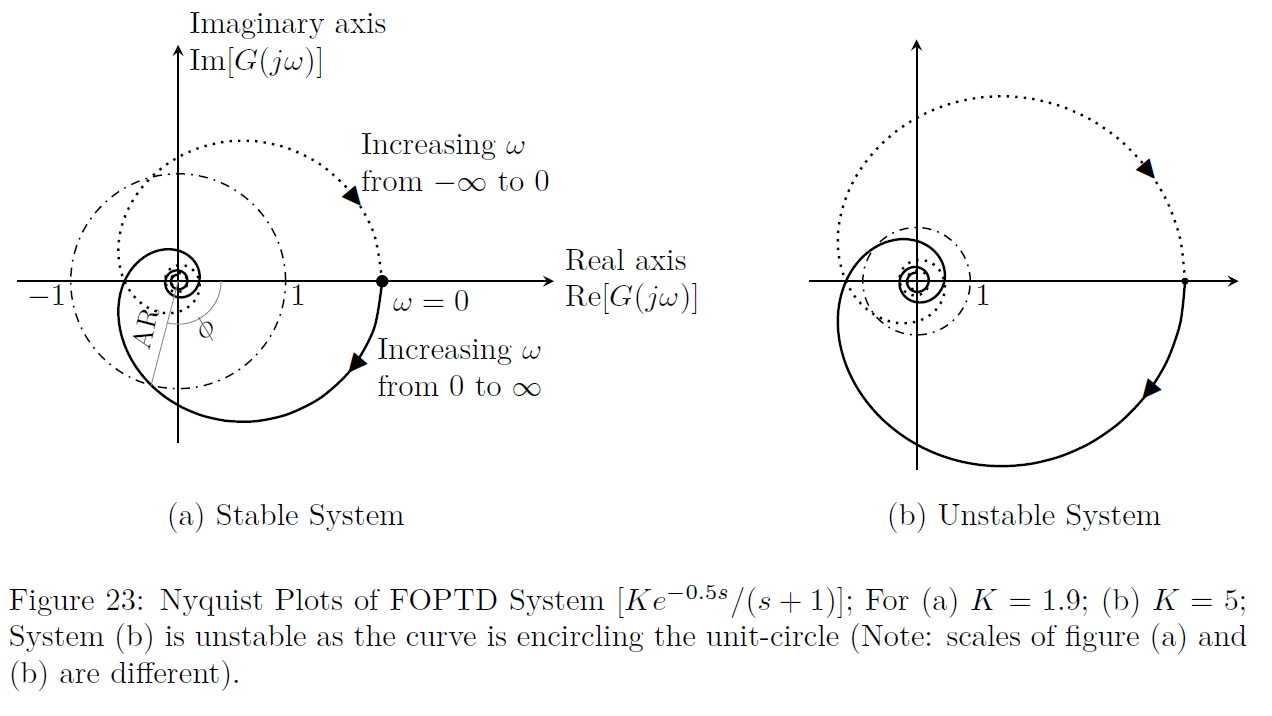
Stability Analysis: Refer to Fig.(23).
The Nyquist stability criterion is given as follows:
“If the open-loop Nyquist plot of a feedback system encircles the point \((-1,0)\) as the frequency (\(\omega\)) takes any value from minus infinity to plus infinity, the closed-loop response is unstable”.
-